Welcome to Software Development on Codidact!
Will you help us build our independent community of developers helping developers? We're small and trying to grow. We welcome questions about all aspects of software development, from design to code to QA and more. Got questions? Got answers? Got code you'd like someone to review? Please join us.
How to pivot text?
In this Q a user asked for a simple way to represent this data:
- PERSON 1 | PERSON 2 | YES
- PERSON 1 | PERSON 3 | YES
- PERSON 2 | PERSON 1 | YES
- PERSON 2 | PERSON 3 | YES
- PERSON 3 | PERSON 1 | NO
- PERSON 3 | PERSON 2 | NO
in this format:
- _________| PERSON 1 | PERSON 2 | PERSON 3 |
- PERSON 1 |   X      |   YES    |    YES   |
- PERSON 2 |   YES    |   X      |    YES   |
- PERSON 3 |   NO     |   NO     |    X     |
This formula was offered as a solution:
=ARRAYFORMULA({{""; UNIQUE({FILTER(A:A,A:A<>"");FILTER(B:B,B:B<>"")})}, {TRANSPOSE(UNIQUE({FILTER(A:A,A:A<>"");FILTER(B:B,B:B<>"")}));IFERROR({ VLOOKUP(UNIQUE({FILTER(A:A,A:A<>"");FILTER(B:B,B:B<>"")}), FILTER(A:C,B:B=INDEX(UNIQUE({FILTER(A:A,A:A<>"");FILTER(B:B,B:B<>"")}),1,1)),3,0), VLOOKUP(UNIQUE({FILTER(A:A,A:A<>"");FILTER(B:B,B:B<>"")}), FILTER(A:C,B:B=INDEX(UNIQUE({FILTER(A:A,A:A<>"");FILTER(B:B,B:B<>"")}),2,1)),3,0), VLOOKUP(UNIQUE({FILTER(A:A,A:A<>"");FILTER(B:B,B:B<>"")}), FILTER(A:C,B:B=INDEX(UNIQUE({FILTER(A:A,A:A<>"");FILTER(B:B,B:B<>"")}),3,1)),3,0)}, "X")}})
where it has been assumed the source table (unlabelled) starts in A2.
A mere copy/paste of a formula written for one is about the simplest possible solution, but, because of formatting, just copy pasting the above may not work. Also, without adjustment, the formula would break if ColumnsA:B were labelled, or might break in case of further content of a different nature in those columns. In addition, the question was tagged [google-sheets-query].
Is there a more memorable way to achieve the desired result, preferably using Google's Query Language?
2 answers
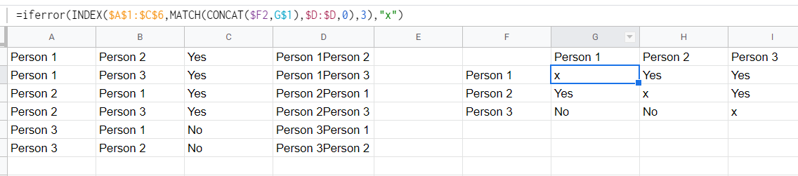
This seems to be looking at the outcome of a bracket in which successive players show an outcome. The table can be easily created by looking at each combination of players and listing them in the table using the index-match combination to find the correct value. Combinations that are not found in the table will return a #N/A error, and we can use iferror to show an exception.
The formula in column D should be a simple concatenation of the values in columns A and B:
=A2&B2
The formula in the top left cell of the table should should be:
=iferror(INDEX($A$1:$C$6,MATCH($F2&G$1,$D:$D,0),3),"x")
Copy & paste to fill the rest of the cells.
0 comment threads
Perhaps (if a process of several relatively familiar steps is easy to remember) but additional formulae may be appropriate, a little extension to the source data required and some formatting. However, the offered solution only works for at most three states (here YES, NO, and X).
First, add the required additional data. This is the trigger for the Xs, so perhaps a formula in A7 and copied across to B7 of:
=unique($A2:$A7)
Enter 0 in ColumnD of each of the rows populated by the UNIQUE formula.
In D2 and copied down (say by double-clicking the fill handle):
=IF(C2="YES",1,-1)
Then in say F2:
=query(A2:D10,"select A, sum(D) group by A pivot B")
Finally for presentation purposes select from ColumnF and to the right and Format > Number > More Formats > Custom number format and:
"YES";"NO";"X"
and Apply.
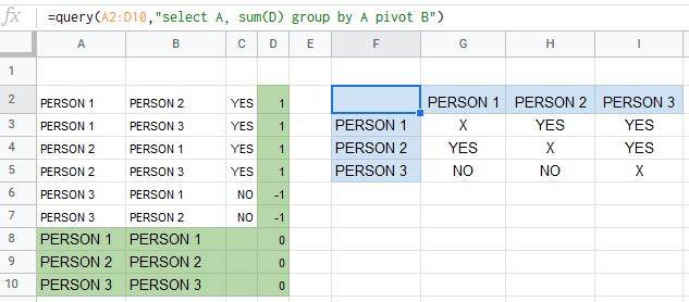
This is extensible for more people (possibly most easily by inserting rows at the position of the UNIQUE formula) but would then require additional population of ColumnD and extending the Query range.
The process would be much simpler if a fill (could be applied with Conditional Formatting) was allowed instead of the Xs and would be easier to extend if a blank row were allowed in the pivot table under its headings.
0 comment threads

1 comment thread